Next: Keyword LPCONSERVE Up: Born-Oppenheimer Molecular Dynamics Previous: Keyword TRAJECTORY Contents
| ANALYZE | A BOMD (property) calculation is analyzed. | ||
| CALCULATE | A property calculation along a BOMD trajectory is requested. |
| DIPOLE | Dipole moments are calculated along a BOMD trajectory. | ||
| POLARIZABILITY | Polarizabilities are calculated along a BOMD trajectory. | ||
|
NMR= | NMR shieldings are calculated along a BOMD trajectory.
The | ||
| MAGNETIZABILITY | Magnetizabilities are calculated along a BOMD trajectory. |
| MOMENTA | Linear and angular molecular momenta are calculated along an MD trajectory. | ||
| PHASESPACE | The reduced coordinate and momentum are calculated along an MD trajectory. This option is valid only for dimers. |
| RDF=A1-A2 | Calculate the radial distribution function between atom A1 and atom A2. | ||
| SIMILARITY | Calculate the similarity index along an MD trajectory with respect to pattern geometries. | ||
| LINDEMANN | Calculate the Lindemann parameter for an MD trajectory. | ||
| MEANDIS | Calculate the mean interatomic distance along an MD trajectory. | ||
| PROLATE | Calculate the prolate deformation parameter along an MD trajectory. |
| LENGTH | Calculate the specified bond lengths along an MD trajectory. | ||
| ANGLE | Calculate the specified angles along an MD trajectory. | ||
| DIHEDRAL | Calculate the specified dihedral angles along an MD trajectory. |
| E=STANDARD | Standard output for the energy analysis of a trajectory file. | ||
| E=KINETIC | The kinetic energy is averaged in the energy analysis of a trajectory file. | ||
| E=POTENTIAL | The potential energy is averaged in the energy analysis of a trajectory file. | ||
| E=TOTAL | The total energy is averaged in the energy analysis of a trajectory file. | ||
| E=SYSTEM | The system energy is averaged in the energy analysis of a trajectory file. | ||
|
INT= | Step interval for property analysis or calculation. Default is 1. |
SIMULATION CALCULATE DIPOLE
The corresponding output has the form:
 TIME [FS] X[A.U.] Y[A.U.] Z[A.U.] |MU|[A.U.] <MU>[A.U.] <MU^2>[A.U]

    101.0   .089    .000    .835      .840       .840       .000
    102.0   .092    .000    .839      .844       .842       .002
    103.0   .093    .000    .842      .848       .844       .003
    104.0   .091    .000    .846      .851       .846       .004
    105.0   .088    .000    .850      .854       .847       .005
    106.0   .083    .000    .852      .856       .849       .006
    107.0   .076    .000    .855      .858       .850       .006
    108.0   .068    .000    .871      .874       .853       .010
    109.0   .060    .000    .864      .866       .855       .010
    110.0   .051    .000    .868      .870       .856       .010
For each time step, the instantaneous dipole moment components and the
corresponding absolute dipole moment are listed, together with the average
value and the standard deviation. The BOMD polarizability [33]
output is similar and discussed in more detail in example ![[*]](crossref.png) on
page of the tutorial.
on
page of the tutorial.
A BOMD property calculation can be specified further by the corresponding
property keyword. Note that NMR shieldings along BOMD trajectories are only
printed for the atom specified by the NMR option of the SIMULATION keyword,
even though all shieldings are calculated by default. To obtain the NMR
shielding for a specific atom use SIMULATION ANALYZE NMR=![]() Integer
Integer![]() , where
, where
![]() Integer
Integer![]() denotes the number of the desired atom in the GEOMETRY definition.
The following input example,
denotes the number of the desired atom in the GEOMETRY definition.
The following input example,
 TRAJECTORY RESTART PART=10-100 INT=1
 SIMULATION ANALYZE NMR=3 INT=1
 GEOMETRY CARTESIAN
 O    0.0000    0.0000    0.1173  17.0
 H    0.0000    0.7572   -0.4692
 H    0.0000   -0.7572   -0.4692
generates an NMR shielding output for atom 3, here the second hydrogen of the water molecule, from trajectory step 10 to 100. Note the TRAJECTORY RESTART option that is used to address only a part of the trajectory file. Besides the detailed NMR shielding information (tensor diagonal elements, instantaneous shielding and averaged shielding) for the specified atom, the corresponding output lists also the NMR shielding statistics for all atoms.
 **********************************************
 *** MOLECULAR DYNAMICS TRAJECTORY ANALYSIS ***
 **********************************************


                   NMR SHIELDING [ppm] FOR ATOM 3

 TIME [FS]      XX       YY       ZZ      SIGMA   <SIGMA>

     10.0      24.73    40.58    31.27    32.19    32.19
     11.0      24.01    39.42    29.88    31.11    31.65
     12.0      23.23    37.98    28.70    29.97    31.09
     13.0      22.70    36.99    28.05    29.25    30.63
     14.0      22.51    36.65    27.96    29.04    30.31
     15.0      22.70    37.04    28.41    29.38    30.16
     16.0      23.27    38.09    29.36    30.24    30.17
     17.0      24.03    39.36    30.52    31.31    30.31
     18.0      24.52    40.04    31.28    31.95    30.49
     19.0      24.36    39.48    31.18    31.68    30.61
     20.0      23.70    38.01    30.44    30.72    30.62
       :         :        :        :        :        :
     90.0      23.49    37.26    30.88    30.54    30.43
     91.0      23.05    36.30    30.36    29.90    30.43
     92.0      22.85    35.89    30.14    29.63    30.42
     93.0      22.94    36.10    30.29    29.78    30.41
     94.0      23.39    37.12    30.86    30.46    30.41
     95.0      24.27    39.07    31.74    31.69    30.42
     96.0      25.00    40.90    32.05    32.65    30.45
     97.0      24.71    40.92    30.93    32.19    30.47
     98.0      23.72    39.41    29.20    30.77    30.47
     99.0      23.02    38.12    28.13    29.76    30.46
    100.0      22.75    37.57    27.79    29.37    30.45

 *** NMR SHIELDINGS STATISTIC ***

 CHEMICAL SHIELDING FOR ATOM 1 ( O )
 AVERAGE SHIELDING [ppm] =   332.87
 STD DEV SHIELDING [ppm] =    13.06

 CHEMICAL SHIELDING FOR ATOM 2 ( H )
 AVERAGE SHIELDING [ppm] =    30.40
 STD DEV SHIELDING [ppm] =     0.81

 CHEMICAL SHIELDING FOR ATOM 3 ( H )
 AVERAGE SHIELDING [ppm] =    30.45
 STD DEV SHIELDING [ppm] =     1.02
The atoms for which NMR shieldings should be calculated along a BOMD trajectory can be selected with the READ option of the NMR keyword, see 4.8.8. Also the nuclear spin-rotation constant [226] can be calculated along BOMD trajectories as shown by the following input example.
 DISPERSION
 BASIS (AUG-CC-PVDZ)
 AUXIS (GEN-A2)
 SCFTYPE MAX=1000 TOL=0.100E-04
 VXCTYPE OPTX-PBE AUXIS
 TRAJECTORY RESTART PART=10000-12000 INT=20
 SHIFT -0.2
 NMR SPINROT
 SIMULATION CALCULATE NMR=1 INT=20
 #
 # Cartesian coordinates of MD step 410000
 #
 GEOMETRY CARTESIAN ANGSTROM
 F   -66.916797   19.630729  -13.088069    9  18.998000
 H   -67.101518   18.720636  -12.997091    1   2.014000
 C    54.166066  -15.936748    9.958016    6  12.000000
 C    53.957601  -15.619981   11.173715    6  12.000000
 H    54.766661  -16.089846    9.024499    1   1.008000
 H    53.312450  -15.623649   12.049412    1   1.008000
Magnetizabilities [228] are calculated along a BOMD trajectory by the following input line:
SIMULATION CALCULATE MAGNETIZABILITY
Similarly to the spin-rotation constant, the rotational g-tensor [229] can be calculated along BOMD trajectories by specifying MAGNETIZABILITY GTENSOR in the the input.
The options MOMENTA and PHASESPACE are generic to MD simulations and, therefore, have no corresponding property keyword. While linear and angular momentum analyses are general, the PHASESPACE analysis can be performed only for diatomic molecules. In general, MOMENTA and PHASESPACE results probe the MD sampling in detail and are recommended if the calculation of thermodynamic properties from the MD trajectory is the objective. Plots from PHASESPACE outputs are shown in Figure 12.
The RDF, SIMILARITY, LINDEMANN, MEANDIS and PROLATE options are intended to be used in combination with the ANALYSE option to perform the respective analysis on an MD trajectory. The RDF option enables a radial distribution function calculation. It requires two string arguments to specify the atomic pair defining the radial distribution function. According to this specification the RDF for a specific atom pair or for all pairs of an element combination are calculated. Specific RDF options can be set by the RDF keyword (see 4.7.7) as in the following example.
 RDF MAX=2.0 WIDTH=0.01
 SIMULATION ANALYSE RDF=C-H INT=10
 #
 GEOMETRY
 C        1.251600     -0.743355     -0.192056
 O        2.419080      0.016064      0.186570
 C       -0.012609      0.001665      0.300080
 H        3.194749     -0.353196     -0.223934
 O       -0.044331      1.355726     -0.228495
 H        0.628856      1.905515      0.161926
 C       -1.248651     -0.749384     -0.241064
 O       -2.455867     -0.060507      0.201783
 H       -2.338769      0.832194     -0.188720
 H       -0.073137     -0.089445      1.394002
 H       -1.226536     -1.787913      0.146590
 H        1.132009     -1.855775      0.371678
 H        1.127880     -0.963356     -1.265091
 H       -1.042307     -0.734311     -1.348578
This input generates an RDF for all C-H distances below 2 Ångström of a glycerol BOMD.
The SIMILARITY option requires the definition of at least one PATTERN geometry. This option triggers the calculation of the normalized RMS distance between the MD and PATTERN geometries which can be used as an index to classify isomers or calculate isomer lifetimes. By default, pattern and MD geometries are aligned (see 4.1.7) before anything is calculated. The automatic pattern-geometry alignment can be modified with the ALIGNMENT keyword if desired. The following input performs a similarity analysis, excluding hydrogen atoms, of glycerol conformers along a BOMD trajectory.
 ALIGN ENANTIOMER EXCLUDE
 H
 SIMULATION ANALYSE SIMILARITY INT=1
 #
 # Pattern definitions
 #
 PATTERN GLYA
 C        0.000000      0.000000      0.000000
 O        0.000000      0.000000      1.462899
 C        1.474005      0.000000     -0.440301
 H       -0.893691     -0.260594      1.766994
 O        2.162480     -1.176562      0.084086
 H        1.941117     -1.214952      1.038194
 C        1.632514     -0.059827     -1.970356
 O        3.025324     -0.048486     -2.363928
 H        3.464920     -0.717132     -1.794492
 H        1.971460      0.922883     -0.056060
 H        1.170832      0.835048     -2.435026
 H       -0.510825      0.910396     -0.391119
 H       -0.502224     -0.913371     -0.392432
 H        1.121602     -0.977513     -2.350343
 PATTERN GLYB
 C        0.000000      0.000000      0.000000
 O        0.000000      0.000000      1.447257
 C        1.448191      0.000000     -0.553309
 H        0.683368      0.660325      1.699576
 O        2.197151      1.114528      0.025822
 H        1.975852      1.886268     -0.546110
 C        1.505454      0.056976     -2.092055
 O        1.020939      1.380454     -2.494249
 H        1.337270      1.554323     -3.403051
 H       -0.524157     -0.927069     -0.313648
 H        2.557147     -0.088302     -2.425107
 H        0.859665     -0.741313     -2.524473
 H       -0.548895      0.882612     -0.405640
 H        1.966016     -0.916375     -0.200050
 GEOMETRY
 C        1.251600     -0.743355     -0.192056
 C        2.419080      0.016064      0.186570
 C       -0.012609      0.001665      0.300080
 O        3.194749     -0.353196     -0.223934
 O       -0.044331      1.355726     -0.228495
 O        0.628856      1.905515      0.161926
 H       -1.248651     -0.749384     -0.241064
 H       -2.455867     -0.060507      0.201783
 H       -2.338769      0.832194     -0.188720
 H       -0.073137     -0.089445      1.394002
 H       -1.226536     -1.787913      0.146590
 H        1.132009     -1.855775      0.371678
 H        1.127880     -0.963356     -1.265091
 H       -1.042307     -0.734311     -1.348578
With the Lindemann option the root-mean-square bond length fluctuation
[230],
@fnswfnvalfnswfalse
##1fnval##1fnswtrue
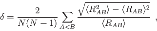 |
(19) |
 |
(20) |
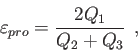 |
(21) |
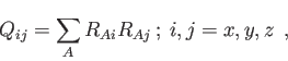 |
(22) |
The LENGTH, ANGLE and DIHEDRAL options require the definition of the atoms involved, in the next input lines. Two numbers are required to define each bond LENGTH, three numbers to define each ANGLE and four numbers to define each DIHEDRAL angle. Up to ten parameters can be defined in this way, in consecutive lines after the keyword, as the following input example shows.
 SIMULATION ANALYSE DIHEDRAL INT=10
 2 1 3 7
 2 1 3 5
 8 7 3 1
 8 7 3 5
 1 5 3 8
 8 3 5 1
 4 5 6 7
 7 6 5 4
 3 1 10 2
 12 11 10 9
 #
 GEOMETRY
 C        1.251600     -0.743355     -0.192056
 O        2.419080      0.016064      0.186570
 C       -0.012609      0.001665      0.300080
 H        3.194749     -0.353196     -0.223934
 O       -0.044331      1.355726     -0.228495
 H        0.628856      1.905515      0.161926
 C       -1.248651     -0.749384     -0.241064
 O       -2.455867     -0.060507      0.201783
 H       -2.338769      0.832194     -0.188720
 H       -0.073137     -0.089445      1.394002
 H       -1.226536     -1.787913      0.146590
 H        1.132009     -1.855775      0.371678
 H        1.127880     -0.963356     -1.265091
 H       -1.042307     -0.734311     -1.348578
The standard energy output of a deMon BOMD run has the following form:
 TIME [FS]  T [K]   EKIN        EPOT        ETOT     <T> [K]   <ETOT>

     10.0   103.5   0.00098  -648.62892  -648.62793   103.0  -648.62793
     20.0   100.3   0.00095  -648.62889  -648.62794   102.7  -648.62793
     30.0    91.4   0.00087  -648.62885  -648.62799   100.2  -648.62795
     40.0    84.9   0.00081  -648.62882  -648.62801    96.8  -648.62796
     50.0    84.2   0.00080  -648.62874  -648.62794    94.2  -648.62797
     60.0   107.4   0.00102  -648.62869  -648.62767    94.3  -648.62794
     70.0   185.8   0.00176  -648.62858  -648.62681   102.2  -648.62784
     80.0   252.2   0.00240  -648.62831  -648.62592   118.8  -648.62763
     90.0   154.0   0.00146  -648.62799  -648.62653   128.2  -648.62747
    100.0    56.3   0.00053  -648.62772  -648.62719   124.2  -648.62742
For each time step it lists the instantaneous temperature, kinetic, potential, and total energy as well as the average temperature and total energy. With the INT option of the SIMULATION keyword, the step interval for the energy output can be modified. Energy statistics along an existing trajectory file can be obtained with:
SIMULATION ANALYZE E=STANDARD
If E=STANDARD is substituted by E=KINETIC, E=POTENTIAL, E=TOTAL, or E=SYSTEM, the averages of the kinetic, potential, total or system2 energies are listed. In the case of E=KINETIC the output takes the form:
 TIME [FS]  EKIN        EPOT        ESYS        ETOT         <EKIN>

     10.0   0.00098  -648.62892  -648.62793  -648.62793     0.0009836
     20.0   0.00095  -648.62889  -648.62791  -648.62794     0.0009680
     30.0   0.00087  -648.62885  -648.62795  -648.62799     0.0009348
     40.0   0.00081  -648.62882  -648.62798  -648.62801     0.0009027
     50.0   0.00080  -648.62874  -648.62788  -648.62794     0.0008821
     60.0   0.00102  -648.62869  -648.62765  -648.62767     0.0009051
     70.0   0.00176  -648.62858  -648.62747  -648.62681     0.0010279
     80.0   0.00240  -648.62831  -648.62741  -648.62592     0.0011989
     90.0   0.00146  -648.62799  -648.62729  -648.62653     0.0012282
    100.0   0.00053  -648.62772  -648.62710  -648.62719     0.0011588
After the trajectory output, energy and temperature statistics are printed. As for
the DYNAMICS keyword, the SIMULATION keyword can be combined with the TRAJECTORY
keyword in order to analyze or calculate properties for parts of a trajectory.